Part III – Predictive Modelling for Collegiate Academic Excellence – An Ongoing Case Study!
Dr. Shree Nanguneri and Co-Author and Project Lead Contributor, Ms. Reethika S. Iyer*

Background:
In Parts I and II, we touched upon the value proposition in understanding the impact of high school on final examination performance. We concluded with results and discussions from our 3-year pilot study (2009-2011) that there is significant variation “within” students in a given high school (India City Case Study) as well as “between” variation across high schools in our pilot study. The secondary conclusion (even though this is an isolated study compared to the nation’s census on tuition fee and academic value) also concurs with the posted survey that a significantly higher student academic performance doesn’t translate to a higher tuition fee.
In Part III, we are focusing on the academic performance at the collegiate level. The objectives include – Students…:
- Are capable of predicting their performance in classes!
- Spend less time toward their studies as they have a predictive model
- Have more downtime in a given day by improving their study strategy
- Invest gained time toward improving their life skills
- Reduce investment for education, and significantly increase chances of employment
- Eliminate less than expected performance or failure in college courses
- Succeed in their internships by applying their problem solving tools
Tuition Fee Structure of Schools and Colleges:
While assessing college tuition compared with that of high school (in India), it is shocking to see that the former is actually significantly less in cost. One of the primary reasons being high school capacity in major metropolitan cities is much less than the demand for children trying to get admitted.
The demand-to-capacity ratio (DCR) is also >1 in colleges, however, as new colleges are opening up by the year compounded by governmental regulations restricting tuition increase, colleges cannot leverage the high DCR values to increased revenues.
High schools can elect to increase tuition and revenue, as they have what is called “donation” or “Capitation” fees that can be charged ruthlessly when the DCR values skyrocket. In fact queuing lines were registered in 2010 where parents are lining up to pick up hard copies of application forms for their children’s admission to such high schools. Whatever happened to online application?
Colleges are also finding ways to get around the legal restrictions by charging special fees for anything they can classify as “out of the norm” justifying the need for such additional charges going directly into their coffers.
Problem Solving Strategy:
In the Lean Six Sigma (LSS) problem solving methodology, the student candidate at a metro city engineering college bore the following demographics:
- City Type – Metropolitan
- High School Classification – Central Board (Federally Controlled)
- High School Medium of Instruction – English
- College Medium of Instruction – English
- College – Private (Deemed University)
- Level – Bachelor of Technology (B. Tech) Sophomore & Junior Years
- Average Class Size – 50 students
- Class Environment – Male and Female
- Major Area of Specialization – Information Technology (IT)
The key realization in this study was very much in line with the foundation of the LSS – DMAIC approach where the output is expressed as a function of the inputs as listed below:
Output Y = Semester Final Grade or Performance
Inputs Xs:
- Proactive Semester Syllabus Validation [C]
- Acquire the prescribed text books and study materials prior to semester kick off [C]
- Compile question papers and question bank of prior years [C]
- Analyze such questions and parse them into frequent and rare types [C]
- Interact with faculty and seniors at a constant basis [P]
- Take mock tests to keep emotional decisions in students’ preparation plans [C]
- Ensure fundamentals are learned well
- Formula sheet for Math type questions
- Programming language for easy references
- Leverage the net and browse question bank of other universities as well [C]
- Using the resources above predict question that is likely to occur [C]
- Take exam on predicted questions [C]
- Predict scores based on trial testing [C]
- Revisit performance, check gaps and perform a root cause analysis [P]
- Improvise model based on surprises to date [P]
- Content of actual test or model or final exam [N]
Results and Discussions:
In this section prior to case study conclusions, we encourage students all over the world that this is translatable across cities, countries and continents even if the system is widely different from each other as we analyze it globally.
The figures, illustrations, and statistical interpretations provided here along with practical explanations are based on hard data compiled that can be validated if needed. There are four process categories as shown below that either help or actually contribute toward the student’s GPA (grade point average):
- Cycle Tests (tests that occur at some point in time (at least twice a semester)
- Short Term testing which is similar to that of a mid-term and
- Henceforth please read it as Surprise Test instead of Short Term (a minor correction)
- A model examination to help student simulate the finals and finally,
- The actual examination performed by student known to them as “finals”
Performance Measures and Metrics:
The college environment conducts a variety of testing environments as shown below:
- Cycle Tests (Occur twice a semester reviewing portions to date)
- Surprise Test (Similar to an assignment or surprise quiz)
- Model Examination (Simulates the Semester Finals)
- Final Semester Examination
- Not part of this analysis as scores are not reported to students
Since each of these testing environments bear a different characteristic such as:
- Length (Time)
- Content (Portion in Syllabus)
- Grading Methodology (multiple choice, partial scores)
- Distribution of Category of Question Types (Short vs Long Answer)
- Grading Professor (Measurement System)
- Total Possible Score (10, 15, 50, or 100)
Looking at the absolute values would not give us a fair or apples-to-apples evaluation and so we have chosen to use the “Standardized Residual” (SR) as our universal metric in our mathematical modelling process.
The SR value corresponding to each test opportunity is obtained as follows:
- Calculate the:
- Residuals (ri) for all 1st cycle tests across 3 semesters (Predicted – Actual)
- One gets either a positive or negative value
- Residuals (ri) for all 1st cycle tests across 3 semesters (Predicted – Actual)
- Average of all residuals (μ)
- Standard Deviation using all residuals (σ)
- SRi = (ri – μ)/σ
- Repeat the process for all other categories:
- 2nd Cycle Test
- Surprise Test
- Model Examination
Since we are combining all testing categories, we choose to utilize the Median of SR as a measure of effectiveness of the students’ predictive model. For effective predictive models the preferred outcome is SR values:
- Follow a normal distribution.
- Range preferably between ± 2.0.
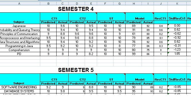
Table 1: Data Structure Sample (Partial View Only):
Graphical Illustrations:
Overall Evaluation:
Figure 1: Overall Dotplot of SR Values across All Testing Categories
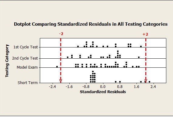 It can be seen in Figure 1 that the SR values in one instance on the model exam and the short term actually exceed the threshold of ± 2.0. Digging deeper, one can analyze and determine if it was a special or common cause that caused this variation.
Each testing category was analyzed to check if their SR values followed a normal or non-normal distribution. For brevity, we will demonstrate two examples (one normal and the other non-normal) and tabulate all test categories in a simple table.
Figure 2: Normality Test for all Model Examinations (Semesters 4, 5, and 6)
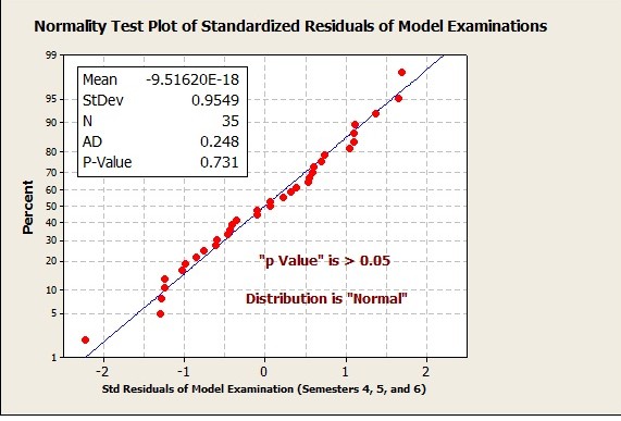 When the “p” value is 0.731 which is > 0.05 as in Figure 2 for Model Examinations, the distribution is regarded as normal (symmetric, or Gaussian). In all statistical evaluations and process characterization, we recommend the use of the “mean” value of SR. There may be reasons for this behavior (which is not the scope of this article, refer to full technical publication coming out this summer).
Figure 3: Normality Test for all 1st Cycle Test Categories (Semesters 4, 5, and 6)
In Table 2 below, we have summarized the characteristics of all test category:
Table 2: Normality Test Characteristics of all Testing Categories
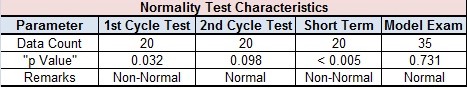
Note: The Model Examination included had 5 semesters of data points versus 3 for other categories.
Figure 3: Normality Test for all Model Examinations (Semesters 4, 5, and 6)
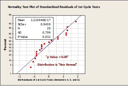 When the “p” value is 0.032 which is < 0.05 as in Figure 3 for 1st Cycle Test, the distribution is regarded as non-normal (asymmetric, or Non-Gaussian). In place of using the “mean” to characterize the process, it is recommended to replace it by the median. There may be reasons for non-normality (which is not the scope of this article, refer to full technical publication coming out this summer).
Figure 4: Overall Graphical Summary of SR Values Across All Testing Categories
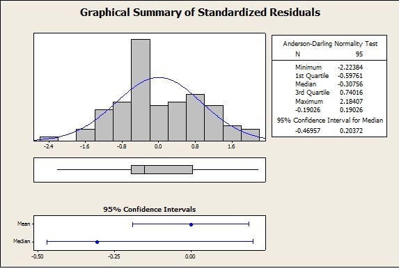 In this analysis we see that the SR values range between -2.22 and + 2.18 (slightly beyond the threshold on both sides).
A + ve value of SR indicates that the student has predicted a score that is higher than the actual value while a – ve value of SR indicates vice versa. If the student had achieved all or a majority of SR values > 0 or < 0, it could then indicate that there is a bias toward the model. In this scenario there seems to be an even distribution with the median SR at -0.3. This means that 50 % of the SR values are above and below -0.3.
The Confidence Intervals on the Median are between -0.5 and +0.2 and this means when the student continues to take any test in the future across semesters without changing the test preparation strategy, there is only a 5 % risk that the median of all SR values will fall outside of this range (-0.5 to + 0.2). There is 95 % confidence, that the student will achieve a SR Median value to fall between -0.5 and +0.2.
Overall Predictive Capability:
The overall predictive capability can be estimated by assuming that the SR values need to fall within the ± 2.0 limits. By plotting the capability of all SR values we can estimate the actual defect rate and quantify the effectiveness of such a model.
Figure 5: Overall Predictive Process Capability across All test Categories
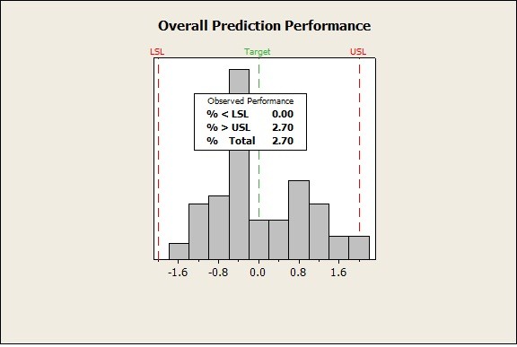
In this case we are looking at 74 instances of test evaluations. The data follows a non-normal distribution and so we assess the predictive capability by looking at the actual defect rate based on the ± 2.0 limits. We see that there are defects on the upper side of the distribution meaning that the predictive model tends to predict 2.7 % more than what the actual score is. Further investigation into those instances of SR values > + 2 can lead to the root causes for the same.
Predictive Process Stability:
The stability of the predictive model can also be viewed by looking at a individual type control chart across all categories and looking for any special causes on the SR values.
Figure 6: Overall Predictive Process Stability Across All Test Categories
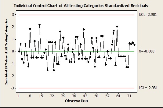
In the individual control chart below Figure 6, we can see that there are no points seeming to be out of control (the standard ± 3s control limits. This also tells us that the predictive model is stable across time as well as categories as these data points are plotted as a function of semester time in the order they occurred.
Correlation and Causation:
The final aspect of our analysis is to understand if there is a correlation and causation between the predicted and actual values of the absolute scores in each category. We will establish one example of correlation and then summarize all correlation coefficients into a simple format as shown in Table 2 below.
Figure 7: Pearson Correlation Coefficient for 1st Cycle Test Category
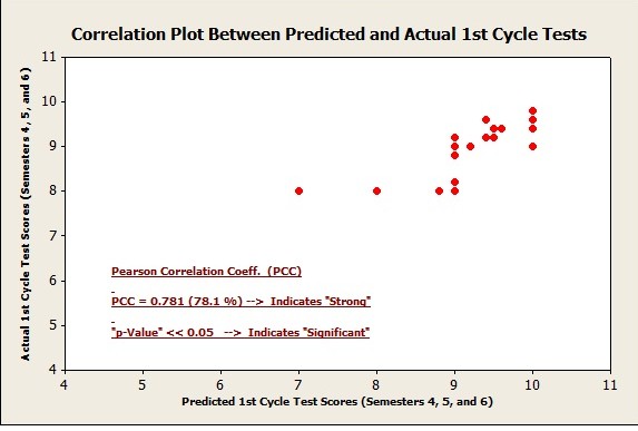
The associated Pearson Correlation Coefficient (PCC) and “p” values are summarized below in Table 3. A “p Value” < 0.05 indicates significance in correlation and a high percentage in PCC also shows a strong correlation.
Table 3: Pearson Correlation Coefficient for All Test Categories
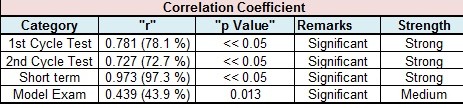
In this predictive modelling there is a causation for this effect as the student is planning and preparing for an output in score based on the controllable and procedural type inputs that they manage proactively. The predictive scores are presented prior to the testing event to eliminate bias in the model. All PCC values indicate between a medium and strong correlation. The “p Values show their statistical significance given that they are < 0.05.
Conclusions:
In conclusion between Parts I-III of this series on PMP and LSS skills in a high school and collegiate environment, there are several opportunities where the simple application of such tools and techniques can bring significant academic and professional value.
On the High School environment that was discussed primarily in Parts I and II, we can envision significant benefits for parent, student and teachers within the institution. Some significant findings point to the age-old hypothesis of whether high tuition fees necessarily mean higher academic value. The pilot study in this series begs for translating the analyses to other metropolitan cities as well as other countries where data transparency is high. The pilot study requires that the final board examination results be published and shared (without revealing student demographics).
The predictive process on the other hand for collegiate students to plan, prepare and execute their academic commitments in a proactive manner is established by having a mathematical model tested and validated. Time is of the essence for a college student and any extraction in a days’ capacity to get more done is appreciated. Moreover, when they are not dragged down in their academic commitment and have a better idea and confidence in their expected performance, they can attend college classes with an aim to improve their critical thinking as opposed to knowledge assimilating. The classroom is no more a nerve centre for gaining knowledge given the benefit of internet access 24-7. The environment is for people coming together to increase their knowledge of the culture of the thought process with their peers and sharpen their critical thinking while polishing their analytical skills.
We plan to convert such models into an application that can be made available to parents for children in high schools as well as college. Models are also being developed for graduate students toward a better performance in their thesis and dissertation outcomes. How does one know if their research has quality on a global measure regardless of where they publish or operate from?
Acknowledgments:
The authors and project lead contributor sincerely thank this audience as well as all other resources for the support and encouragement offered in completing this high school pilot study as well as the predictive modelling in a college environment. Without the efforts of such a team, this work and the results achieved would have only been a pipe dream.
About the Authors
Ms. Reethika S. IyerI am a 3rd year undergraduate studies (B. Tech) student at SRM University, Chennai (India) majoring in the field of Information Technology (IT). One of my current key areas of research interests is “High School and Collegiate Student Performance Excellence” in India. This internship project aims at quantifying the relationship between the choice of high school in India and its impact on a student’s short and long term career. I have been fortunate to be mentored and coached by Dr. Shree Nanguneri, CEO, MGBS Inc. In this internship at MGBS, India, I have acquired a few critical Project Management and Planning (PMP) and Lean Six Sigma (LSS) problem solving skills which I have used in different areas (From planning for higher studies to predicting grades at college). In future I will be executing projects at higher level of complexity that will have a social significance at a global level which excites me professionally as well as provides an opportunity to significantly contribute to the society and make a difference. I plan to adapt to a professional career applying the skills of PMP, LSS, and IT while in parallel, pursuing my higher studies in the field of business administration. |
Dr. Shree NanguneriI am a business process improvement coach and consultant and have worked with several corporations in different continents over the last two decades. After having a successful 6-year work experience at GE, I started my own consulting company in 2000. I have been fortunate to successfully deliver across a variety of industries that include the fields of manufacturing, transactional as well as service type environments. I have published a few articles, authored patents and releasing a book in mid 2011. Although not an expert, I can converse reasonably well in Dutch, and Spanish, skills I acquired while working there. To date, the total annualized direct customer benefits from my services have accrued to several hundreds of millions of dollars. I enjoy outdoor activity, meeting people on a global level to mutually benefit each other. I am also thankful to my mentor as well as network members without which some of the achievement listed here would have been impossible. |
